From Prompt to Token: How LLM Inference Actually Works
You type a question. A second later, words start appearing. Between your keypress and that first token lies a pipeline that most practitioners never examine. This is what happens inside the model during that second.
Every conversation with an LLM follows the same invisible sequence. Your text becomes numbers. Those numbers pass through dozens of transformer layers. A probability distribution emerges. A single token is selected. That token is appended to the input, and the whole process repeats.
The result feels like fluent thought. The mechanism is matrix multiplication.
This article walks through the inference pipeline from end to end, from the moment your prompt enters the model to the moment a token is selected and returned. Not training. Not fine-tuning. Just the forward pass and the sampling decision that follows it.
The Pipeline at a Glance
Before diving into each stage, here is the full sequence. Every token a language model generates follows these steps:
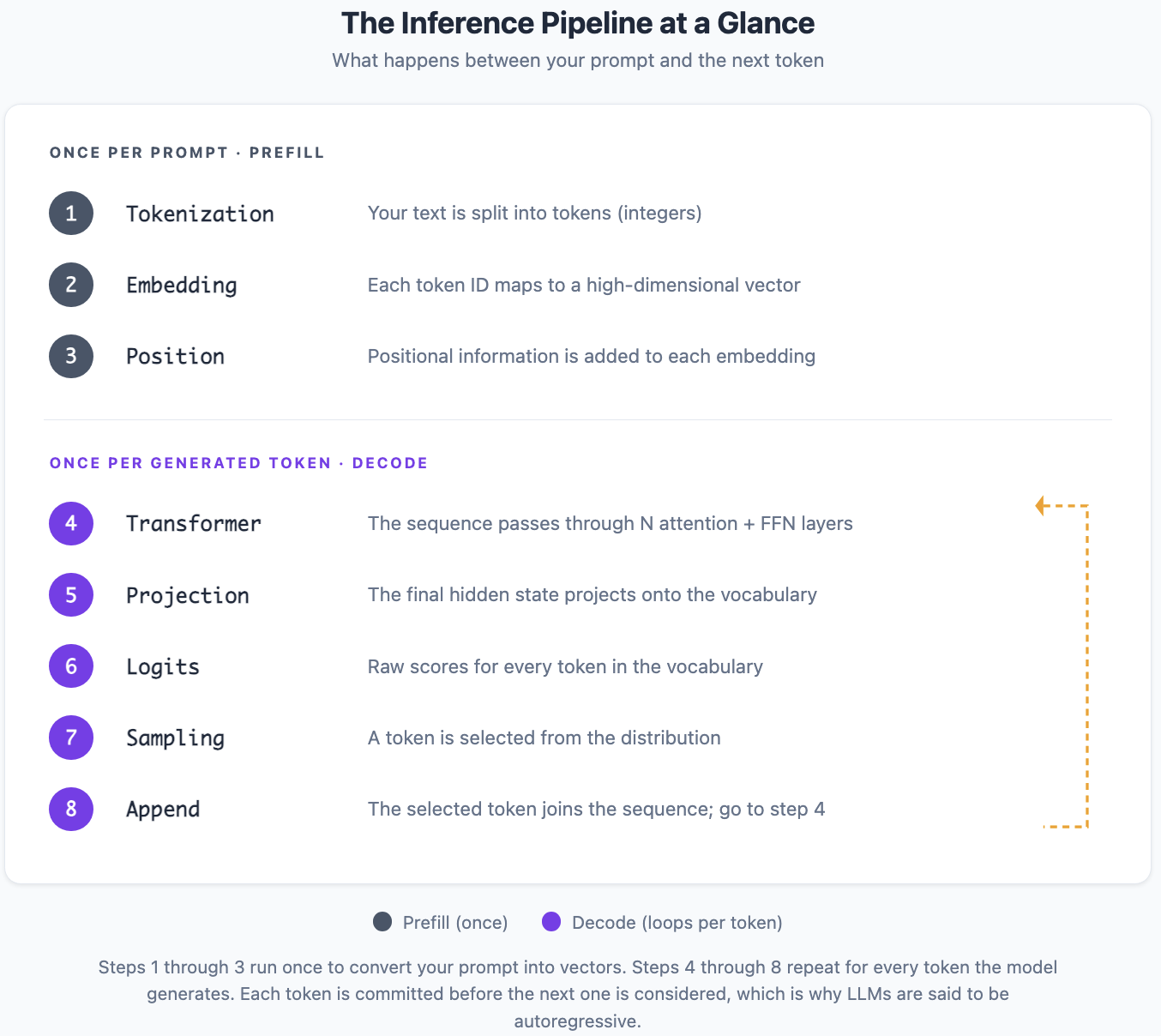
Steps 1 through 3 happen once per prompt. Steps 4 through 8 repeat for every token generated. The model doesn't plan ahead. It doesn't draft a sentence and then type it out. It commits to one token at a time, and each choice constrains every future choice.
This is autoregressive generation, and it is the only mode of operation for decoder-only models like GPT-4, Claude, and LLaMA.1
Step 1: Tokenization
The model doesn't see text. It sees integer sequences. Tokenization converts your prompt into those integers.2
Byte Pair Encoding (or a close variant) splits your input into subword tokens, each mapped to an integer. The details of how BPE works are covered in depth elsewhere. What matters here is the output: a list of token IDs.3
↗ docsimport tiktoken

enc = tiktoken.encoding_for_model("gpt-4")
tokens = enc.encode("The cat sat on the mat")

print(tokens)
# [791, 8415, 9107, 389, 279, 2402]

print([enc.decode_single_token_bytes(t) for t in tokens])
# [b'The', b' cat', b' sat', b' on', b' the', b' mat']
Six words become six integers. Each integer is an index into the model's vocabulary, typically 32,000 to 128,000 entries. This is the only representation the model ever works with. From this point forward, "The cat sat on the mat" is [791, 8415, 9107, 389, 279, 2402].4
The tokenizer also prepends any special tokens the model expects. Some architectures use a <bos> (beginning of sequence) token. Chat models wrap your message in role markers. The system prompt, conversation history, and your latest message are all concatenated into a single token sequence before the model sees any of it.
Step 2: Embedding Lookup
Each token ID indexes into an embedding matrix. This is a simple table lookup, not a computation.
If the model has a vocabulary of 100,000 tokens and a hidden dimension of 4,096, the embedding matrix is a 100,000 x 4,096 table. Token 8415 ("cat") retrieves row 8,415. The result is a vector of 4,096 floating-point numbers.5
# Conceptually:
embedding_matrix = model.embed_tokens.weight  # shape: [vocab_size, hidden_dim]

token_id = 8415  # "cat"
vector = embedding_matrix[token_id]  # shape: [4096]
This vector is the model's initial representation of the token. It knows nothing about context yet. The vector for " cat" is the same whether the sentence is "The cat sat on the mat" or "The cat exploited a zero-day vulnerability." Context comes later, in the attention layers.
The embedding is a learned parameter. During training, gradient descent adjusted these 4,096 numbers so that tokens appearing in similar contexts end up with similar vectors. But this is a static embedding, a single point in high-dimensional space representing the average of all contexts the token appears in. Contextual disambiguation happens in the transformer layers, not here.6
Step 3: Positional Encoding
Attention is permutation-invariant. Without positional information, the model cannot distinguish "The cat sat on the mat" from "mat the on sat cat The." Every token would relate to every other token with no sense of order.
Positional encoding solves this by adding position-dependent information to each embedding vector.
The Original: Sinusoidal Encoding
The 2017 "Attention Is All You Need" paper used fixed sinusoidal functions. Each position in the sequence gets a unique pattern of sine and cosine values across the embedding dimensions:
Position 0 gets one pattern. Position 1 gets a different pattern. Position 1000 gets yet another. The key property is that the relative distance between any two positions can be computed from their encodings. The model can learn "token at position 5 is three positions after token at position 2" without being explicitly told.7
These encodings are added to the token embeddings, not concatenated. The vector for " cat" at position 1 is the sum of its embedding vector and the positional encoding for position 1.8
Modern: Rotary Position Embeddings (RoPE)
Most current models use Rotary Position Embeddings, introduced by Su et al. in 2021. Instead of adding a positional vector, RoPE rotates the query and key vectors in the attention mechanism by an angle proportional to their position.
The mathematical detail matters less than the practical consequence: RoPE encodes relative position directly into the attention computation. When token A attends to token B, the attention score naturally incorporates how far apart they are in the sequence. This makes the model better at generalizing to sequence lengths it didn't see during training, which is why RoPE has become standard in LLaMA, Mistral, and most open-source models.910
Step 4: The Transformer Layers
This is where inference spends most of its time. The sequence of embedded, position-encoded vectors passes through a stack of identical transformer layers. GPT-3 has 96 layers. LLaMA 2 70B has 80. Each layer has two sub-components: multi-head self-attention and a feed-forward network.
Multi-Head Self-Attention
Attention is the mechanism that lets each token look at every other token in the sequence and decide what information to incorporate. The detailed mechanics of Q-K-V attention are covered in depth elsewhere. Here is the summary relevant to inference.
For each token in the sequence, the model computes three vectors from the current representation:
- Query (Q): "What information am I looking for?"
- Key (K): "What information do I contain?"
- Value (V): "What information do I contribute?"
The attention score between two tokens is the dot product of one token's query and another's key, scaled by the square root of the key dimension:
The softmax turns raw dot-product scores into a probability distribution. Each token ends up with a weighted blend of all other tokens' value vectors, where the weights reflect relevance as determined by query-key matching.11
"Multi-head" means this computation happens in parallel across multiple independent attention heads (32, 64, or 128 depending on the model). Each head learns to attend to different types of relationships. One head might specialize in syntactic dependencies ("subject attends to its verb"). Another might track positional patterns ("this token attends to the token two positions back"). Yet another might handle semantic associations ("oracle" attending strongly to "Neo").
The outputs of all heads are concatenated and projected back to the model's hidden dimension.1213
The Causal Mask
During inference, a crucial constraint applies: each token can only attend to tokens at its position or earlier in the sequence. It cannot look ahead. This is enforced by a causal mask that sets future-position attention scores to negative infinity before the softmax, driving their weights to zero.
This is what makes the model autoregressive. When generating token 50, the model can see tokens 1 through 49. It cannot see tokens 51 and beyond because they don't exist yet. The model must commit to token 50 before it can consider what comes after.
A 5-token causal mask: rows are query tokens, columns are key tokens, and a token may only attend to itself and what came before.
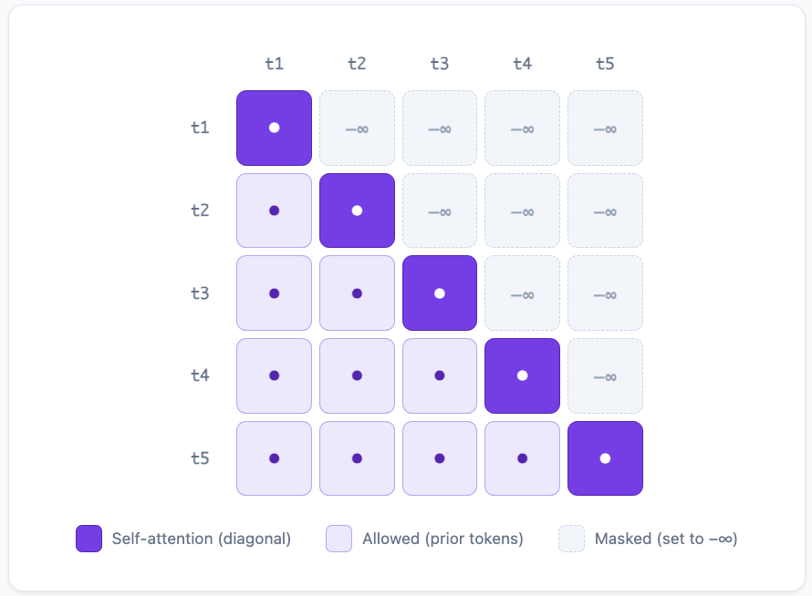
This mask is the fundamental difference between encoder models (like BERT, which see the full sequence bidirectionally) and decoder models (like GPT, which see only the past). Every generative language model uses a causal mask during inference.1415
Feed-Forward Network
After attention, each token's updated representation passes through a position-wise feed-forward network. This is typically two linear transformations with a nonlinear activation in between:
The inner dimension is usually 4x the hidden dimension (so 16,384 for a model with hidden dimension 4,096). This expansion and compression acts as a "memory" step where the model can store and retrieve information learned during training.
Recent research suggests that the feed-forward layers function as key-value memories, where the first linear layer (W1) maps patterns to keys and the second (W2) maps keys to values. When the input matches a stored pattern, the corresponding knowledge is activated. This is where factual knowledge lives in the model: capital cities, programming syntax, mathematical identities.16
Layer Normalization and Residual Connections
Two more components appear in every layer, easy to overlook but essential for stable inference.
Residual connections add the input of each sub-layer to its output. If the attention sub-layer transforms x into Attention(x), the actual output is x + Attention(x). This lets gradients flow directly through the network and allows each layer to learn incremental refinements rather than complete transformations.
Layer normalization (or RMSNorm in many modern architectures) scales the representations to have consistent magnitude. Without it, values would grow or shrink unpredictably across 80+ layers, causing numerical instability.
The combined computation for one transformer layer looks like this:
# Pre-norm architecture (LLaMA, Mistral, most modern models):

x_norm = RMSNorm(x)
x = x + MultiHeadAttention(x_norm)    # residual connection

x_norm = RMSNorm(x)
x = x + FeedForward(x_norm)              # residual connection
This block repeats for every layer. Layer 1 captures simple patterns (word boundaries, common phrases). Layer 40 captures complex relationships (sentiment, logical structure). Layer 80 captures high-level abstractions (argument coherence, stylistic consistency). The representations refine progressively, with each layer building on the work of all previous layers.
Step 5: The Final Projection
After the last transformer layer, we have a hidden state vector for each token in the sequence. For generation, we only care about the hidden state of the last token, because that's where the model's prediction for the next token lives.
This final hidden state is a vector of dimension d_model (e.g., 4,096). To turn it into a prediction over the vocabulary, the model multiplies it by the "language model head," a linear layer that projects from d_model dimensions to vocab_size dimensions:
logits = W_lm_head @ hidden_state_last_token

# W_lm_head shape: [vocab_size, hidden_dim]
# hidden_state shape: [hidden_dim]
# logits shape: [vocab_size]
The result is a vector of raw scores, one per token in the vocabulary. If the vocabulary has 100,000 tokens, you get 100,000 numbers. These are called logits.
In many models, the language model head shares its weights with the embedding matrix. The embedding matrix maps token IDs to vectors (going into the model). The language model head maps vectors back to token scores (coming out of the model). Using the same weights for both is called "weight tying," and it reduces the number of parameters while enforcing a consistent representation.17
Step 6: Logits
Logits are unbounded real numbers. They can be positive, negative, or zero. Their absolute values don't have direct meaning. Only their relative ordering matters.
After the model processes "The cat sat on the," the logits might look something like this:
| Token | Token ID | Logit |
|---|---|---|
| mat | 2402 |
8.7 |
| floor | 4631 |
6.2 |
| table | 2048 |
5.9 |
| bed | 10040 |
5.1 |
| roof | 16244 |
4.3 |
| ground | 5015 |
4.1 |
| couch | 40517 |
3.8 |
| ... | ... | ... |
| quantum | 31228 |
-12.4 |
The actual values are arbitrary; "mat" being 8.7 doesn't mean anything on its own.
A vocabulary of 100,000 tokens produces 100,000 logits. Most are deeply negative. A few dozen are competitive. The model has effectively ranked every possible next token by plausibility, and the top candidates make intuitive sense: surfaces a cat might sit on.
But logits are not probabilities. A logit of 8.7 is not "87% likely." To convert logits into a probability distribution, we need one more step.
From Logits to Probabilities: Softmax
The softmax function converts a vector of logits into a valid probability distribution (all values between 0 and 1, summing to 1):
The exponential amplifies differences. A logit of 8.7 versus 6.2 doesn't look dramatic, but after exponentiation:
exp(8.7)  = 5,982
exp(6.2)  = 493
exp(5.9)  = 365
exp(4.3)  = 74
exp(-12.4) = 0.000004

# After normalization:
P("mat")     ≈ 0.82    # 82%
P("floor")   ≈ 0.07    # 7%
P("table")   ≈ 0.05    # 5%
P("roof")    ≈ 0.01    # 1%
P("quantum") ≈ 0.0000  # effectively zero
"Mat" goes from having the highest logit to dominating the probability distribution. The gap between 8.7 and 6.2 looks modest in logit space. In probability space, it's the difference between 82% and 7%.
This is the distribution the sampling algorithms operate on. Everything that follows is about how to choose a token from this distribution.18
Step 7: Sampling Strategies
Given a probability distribution over 100,000 tokens, how do you pick one?
This is the question that separates a language model (which computes distributions) from a text generator (which produces output). The model's job ends at the logits. Sampling is a separate decision, made outside the neural network, and it profoundly shapes the character of the output.
Greedy Decoding
The simplest strategy: always pick the token with the highest probability.
def greedy_decode(logits):
    return logits.argmax()
One line of code. Deterministic. Given the same input, you always get the same output.
Greedy decoding maximizes local confidence at every step. The model picks the most likely next token, then the most likely token after that, then the most likely after that.
The problem is that local optima don't guarantee global optima. Consider a model deciding between:
- Path A: "The cat sat on the mat" (P=0.82), then "." (P=0.60)
- Path B: "The cat sat on the floor" (P=0.07), then " and purred contentedly." (P=0.90)
Greedy decoding always picks "mat" because 0.82 > 0.07. But Path B might produce a better overall sentence. Greedy can't see that because it never looks ahead.
In practice, greedy decoding produces text that is correct but boring. It repeats common patterns, avoids creative phrasing, and degenerates into loops on longer generations. It's the model equivalent of always ordering the most popular item on the menu.
Beam Search
Beam search addresses greedy decoding's myopia by maintaining multiple candidate sequences simultaneously.
Instead of tracking a single best sequence, beam search tracks the top B sequences (where B is the "beam width," typically 4 to 10). At each step, it expands all B candidates by one token, scores all possible continuations, and keeps the top B overall.
# Beam search with beam width 3:
#
# Step 1: Top 3 next tokens
#   "...the mat"     (score: 0.82)
#   "...the floor"   (score: 0.07)
#   "...the table"   (score: 0.05)
#
# Step 2: Expand each, keep top 3 overall
#   "...the mat."              (0.82 × 0.60 = 0.492)
#   "...the floor and"         (0.07 × 0.90 = 0.063)
#   "...the mat and"           (0.82 × 0.07 = 0.057)
Beam search was the dominant strategy in machine translation for years. It produces higher-quality output than greedy decoding because it considers multiple paths. But it shares a fundamental characteristic with greedy: it is deterministic. Given the same input and beam width, you always get the same output.
For machine translation, determinism is a feature. You want the same French sentence to always produce the same English translation. For creative text generation, determinism is a deficiency. Ask a model to write a poem, and you want different poems each time. Beam search cannot do this.
This is the motivation for stochastic sampling methods.
Temperature
Temperature is the most fundamental sampling parameter. It reshapes the probability distribution before a token is drawn from it.
The mechanism is simple: divide the logits by a temperature value T before applying softmax.
def sample_with_temperature(logits, temperature):
    scaled_logits = logits / temperature
    probs = softmax(scaled_logits)
    return random_choice(probs)
The temperature controls the "sharpness" of the distribution:
| Temperature | Effect on Distribution | Output Character |
|---|---|---|
T = 0.0 |
All probability on the top token | Identical to greedy decoding. Deterministic. |
T = 0.3 |
Very sharp; top 2-3 tokens dominate | Focused, predictable, minimal creativity |
T = 0.7 |
Moderate spread; top 10-20 viable | Balanced coherence and variety |
T = 1.0 |
Raw model distribution, unmodified | Natural model behavior |
T = 1.5 |
Flattened; many tokens competitive | Creative but sometimes incoherent |
T = 2.0+ |
Nearly uniform across vocabulary | Approaching random; mostly nonsense |
on high-scoring tokens. Higher spreads it across more candidates.
Let's trace the math for our "The cat sat on the ___" example:
# Original logits: mat=8.7, floor=6.2, table=5.9, roof=4.3

# T=0.5 (sharp):
# scaled: mat=17.4, floor=12.4, table=11.8, roof=8.6
P("mat")   ≈ 0.99    # almost certain
P("floor") ≈ 0.006
P("table") ≈ 0.003

# T=1.0 (natural):
P("mat")   ≈ 0.82
P("floor") ≈ 0.07
P("table") ≈ 0.05

# T=2.0 (flat):
# scaled: mat=4.35, floor=3.1, table=2.95, roof=2.15
P("mat")   ≈ 0.41
P("floor") ≈ 0.12
P("table") ≈ 0.10
At T=0.5, "mat" is a near-certainty. At T=2.0, the model is almost as likely to pick "floor" or "table." Same logits, same model knowledge, radically different behavior.19
Temperature alone doesn't prevent the model from occasionally selecting tokens with very low probability. Even with a moderate temperature, the distribution has a long tail: 99,990 tokens with near-zero probability, but not exactly zero. On rare occasions, one of those tail tokens will be selected, producing a word that makes no sense in context.
This is where truncation strategies come in.
Top-k Sampling
Top-k sampling restricts the selection to the k highest-probability tokens. All other tokens are excluded by setting their probabilities to zero, and the remaining probabilities are renormalized.
def top_k_sample(logits, k):
    top_k_logits, top_k_indices = logits.topk(k)
    probs = softmax(top_k_logits)
    chosen = random_choice(top_k_indices, probs)
    return chosen
With k=5, only the top 5 tokens are considered. With k=50, the top 50. The model cannot select token 51 or beyond, regardless of its probability.
The problem with top-k is that it's context-insensitive. Sometimes the distribution is sharply peaked (one token has 95% probability), and top-k wastes slots on tokens the model barely considers. Other times, the distribution is flat (many tokens are roughly equally likely), and k=50 might be too restrictive, cutting off viable options.
Consider two situations:
# Situation A: Sharp distribution
# "The capital of France is ___"
#   Paris: 0.97, Lyon: 0.01, Marseille: 0.008, ...
# Top-k=50 includes 47 tokens the model doesn't really want

# Situation B: Flat distribution
# "I went to the ___ for dinner"
#   restaurant: 0.08, cafe: 0.07, diner: 0.06, pub: 0.05,
#   bistro: 0.04, bar: 0.04, steakhouse: 0.03, ...
# Top-k=5 cuts off perfectly good options
A fixed k cannot adapt to both situations. You need something that scales with the distribution's shape.
Top-p (Nucleus) Sampling
Top-p sampling, introduced by Holtzman et al. in 2020, solves this by adapting the cutoff to the distribution. Instead of a fixed count, top-p selects the smallest set of tokens whose cumulative probability exceeds a threshold p.
def top_p_sample(logits, p):
    probs = softmax(logits)
    sorted_probs, sorted_indices = probs.sort(descending=True)

    cumulative = sorted_probs.cumsum(dim=0)
    mask = cumulative <= p

    # Always include at least the top token
    mask[0] = True

    # Zero out excluded tokens, renormalize
    filtered = sorted_probs * mask
    filtered = filtered / filtered.sum()

    chosen = random_choice(sorted_indices, filtered)
    return chosen
With p=0.9, the algorithm includes tokens until their cumulative probability reaches 90%. For "The capital of France is ___," that might be just 1 token (Paris at 97%). For "I went to the ___ for dinner," it might be 15 or 20 tokens.
Top-p adapts automatically to the distribution's shape. When the model is confident, few tokens make the cut. When the model is uncertain, many do. The parameter p controls how much of the probability mass to preserve, not how many tokens to keep.20
Common defaults: p=0.9 (90% of the probability mass) or p=0.95 (95%). At p=1.0, top-p is disabled (all tokens are included).
Combining Strategies
In practice, temperature, top-k, and top-p are often used together. The processing order matters:
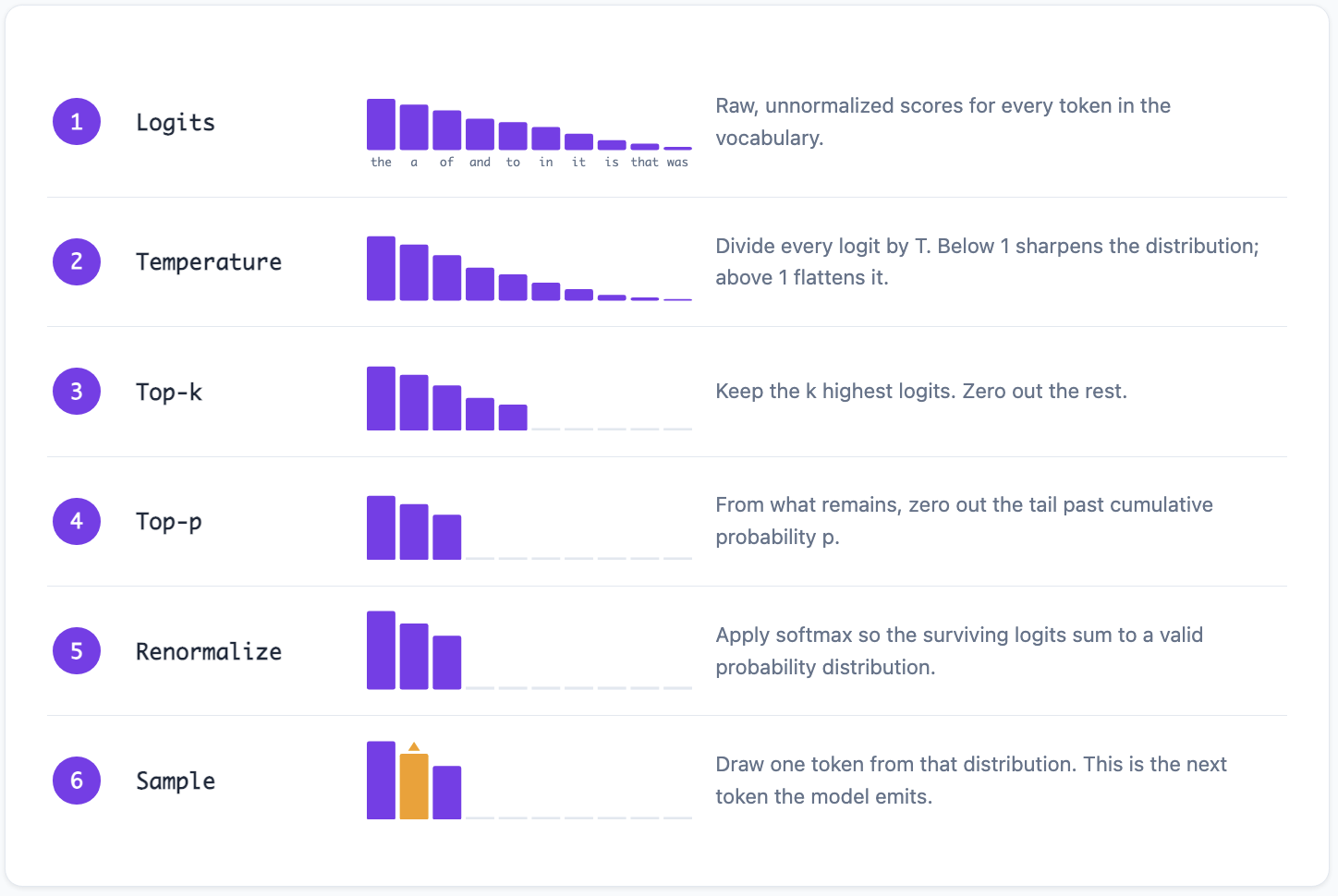
Temperature reshapes the distribution. Top-k and top-p truncate it. The combination provides both shape control and tail removal.
A common production configuration:
| Use Case | Temperature | Top-p | Top-k |
|---|---|---|---|
| Code generation | 0.0 - 0.2 |
0.95 |
disabled |
| Factual Q&A | 0.0 - 0.3 |
0.9 |
disabled |
| General chat | 0.7 |
0.9 |
disabled |
| Creative writing | 0.9 - 1.0 |
0.95 |
disabled |
| Brainstorming | 1.0 - 1.2 |
0.95 - 1.0 |
disabled |
top-p provides adaptive truncation that top-k cannot match.
Top-k has fallen out of favor in most production systems. Top-p provides the same safety (preventing tail selection) while adapting to the distribution's shape. Most API providers don't even expose top-k as a parameter.21
Other Sampling Techniques
Beyond the big three, several other sampling strategies appear in research and specialized applications.
Min-p sampling sets a minimum probability threshold relative to the top token's probability. If the top token has probability 0.82, and min-p is set to 0.1, any token with probability below 0.082 (10% of the top) is excluded. Like top-p, this adapts to the distribution's shape, but it uses a relative threshold rather than cumulative mass. Min-p has gained traction in open-source inference frameworks like llama.cpp and vLLM.
Repetition penalty reduces the logits of tokens that have already appeared in the generated text. This discourages the model from repeating itself, a common failure mode in long-form generation. The penalty typically multiplies the logit of previously-seen tokens by a factor less than 1.0 (or divides by a factor greater than 1.0).
Frequency and presence penalties (as exposed by the OpenAI API) operate similarly but distinguish between how many times a token has appeared (frequency) and whether it has appeared at all (presence). Frequency penalty scales with repetition count; presence penalty applies a fixed reduction for any token that's appeared even once.
Typical sampling (Meister et al., 2023) takes an information-theoretic approach. Instead of selecting the most probable tokens, it selects tokens whose information content (negative log probability) is closest to the expected information content of the distribution. This preferentially selects tokens that are "typically surprising," avoiding both overly predictable and overly surprising choices.
Step 8: The Autoregressive Loop
Once a token is selected, it's appended to the input sequence, and the entire forward pass repeats. The model now processes the original prompt plus the newly generated token, producing logits for the next position.
This is the autoregressive loop:
def generate(model, prompt_tokens, max_new_tokens, temperature, top_p):
    tokens = prompt_tokens

    for _ in range(max_new_tokens):
        # Forward pass: all tokens in, logits out
        logits = model(tokens)

        # Only the last position's logits matter
        next_token_logits = logits[-1]

        # Apply temperature
        next_token_logits = next_token_logits / temperature

        # Apply top-p
        next_token = top_p_sample(next_token_logits, top_p)

        # Append and continue
        tokens = tokens + [next_token]

        # Stop if end-of-sequence token
        if next_token == EOS_TOKEN:
            break

    return tokens
Each iteration generates exactly one token. A 200-word response might require 250+ forward passes, each processing the entire (growing) sequence. This is why inference is computationally expensive, and why techniques like KV-caching (described below) are essential for practical deployment.
The loop terminates when the model produces a special end-of-sequence (EOS) token, when the maximum generation length is reached, or when the model hits the context window limit.
The KV-Cache: Making This Fast Enough
There's a performance problem with the naive autoregressive loop. Each forward pass processes the entire sequence from scratch. Generating token 200 recomputes attention over all 200 tokens, including the first 199 tokens it already processed in the previous iteration.
This is wasteful. The attention computation for tokens 1 through 199 hasn't changed since the previous step (the causal mask ensures that earlier tokens don't attend to later ones). Only the new token's interactions need fresh computation.
The KV-cache exploits this by storing the key and value projections from previous steps. On each new forward pass, the model only computes Q, K, V for the new token. The K and V from all previous tokens are retrieved from cache. The attention computation uses the new token's Q against all cached Ks to compute attention weights, then blends the cached Vs.
Naive decoding, four steps:
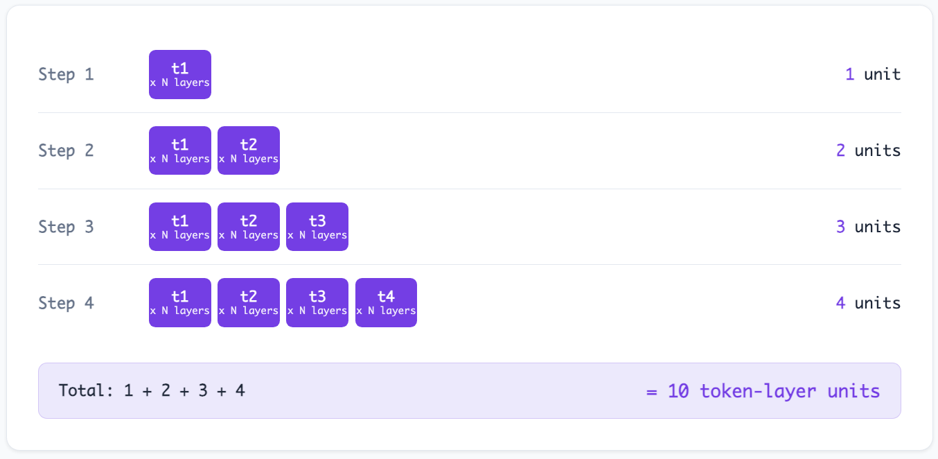
Cached decoding, same four steps:
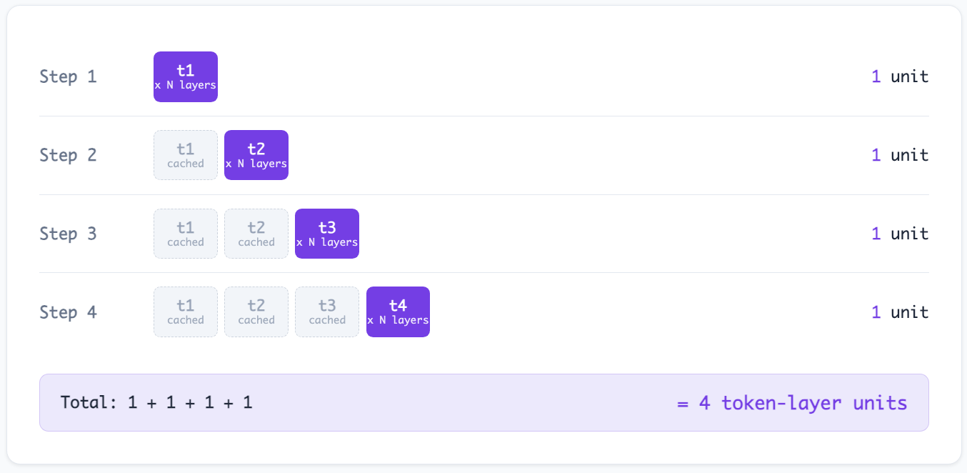
The savings compound with sequence length. For a 2,000-token generation, the naive approach performs roughly 2,000,000 token-layer computations. With KV-cache, it performs roughly 2,000. That's a 1,000x reduction.22
The cost is memory. The KV-cache stores two vectors per token per layer per attention head. For a 70B-parameter model with 80 layers, 64 heads, and a key dimension of 128, the cache for a single 4,000-token sequence consumes:
Memory footprint, factor by factor:
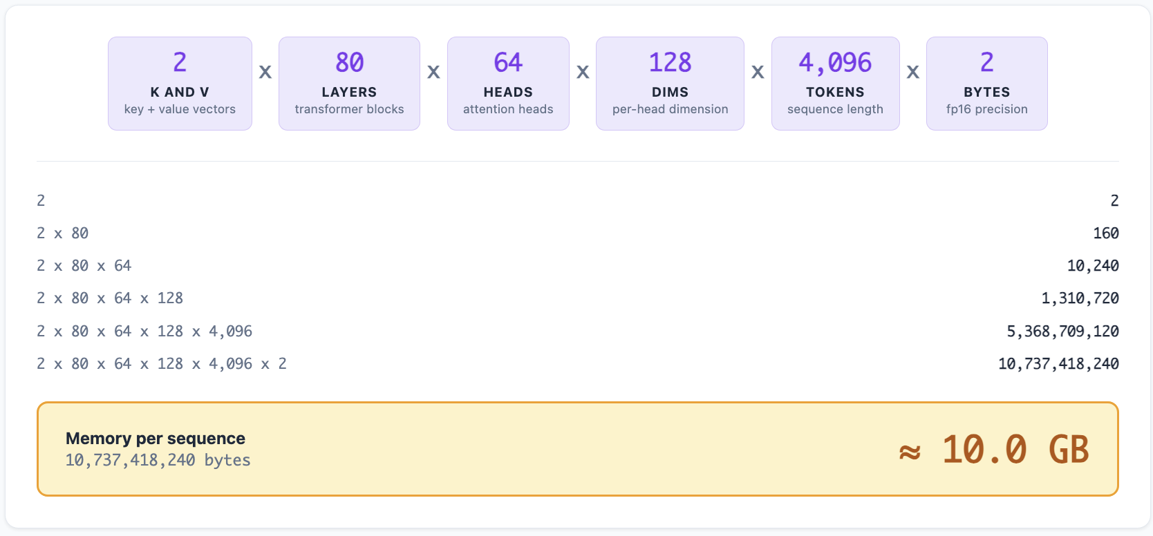
This is why serving large models requires significant GPU memory even beyond the model weights themselves. The KV-cache grows linearly with both sequence length and batch size. Serving 100 concurrent conversations with long context windows can require more memory for the cache than for the model itself.23
The Prefill and Decode Phases
When a request arrives at an inference server, processing happens in two distinct phases with very different computational characteristics.
Prefill (Prompt Processing)
The entire prompt is processed in a single forward pass. All tokens in the prompt are processed simultaneously through all transformer layers. This is compute-bound: the GPU's arithmetic units are the bottleneck. The prompt can be processed in parallel because all tokens are known in advance.
Prefill produces the KV-cache entries for all prompt tokens and generates the logits for the first new token.
Decode (Token Generation)
Each subsequent token is generated one at a time. This phase is memory-bandwidth-bound, not compute-bound. The computation per step is small (one new token), but it requires reading the entire KV-cache from GPU memory, along with all model weights. The GPU spends most of its time waiting for memory reads, not doing arithmetic.
This asymmetry has practical consequences:
| Metric | Prefill | Decode |
|---|---|---|
| Bottleneck | Compute (FLOPs) | Memory bandwidth |
| Parallelism | All prompt tokens at once | One token at a time |
| GPU utilization | High (near peak FLOPS) | Low (memory-bound) |
| Latency profile | Time to first token (TTFT) | Inter-token latency (ITL) |
| Optimization | Flash Attention, parallelism | KV-cache, speculative decoding |
Optimizing them requires fundamentally different strategies.
This is why "time to first token" and "tokens per second" are measured separately. A model might prefill a 4,000-token prompt in 800ms (5,000 tokens/second throughput during prefill) but then generate at only 30 tokens/second during decode. The user perceives a pause before text starts, then a steady stream.
Speculative Decoding
One important optimization deserves mention because it changes the dynamics of the autoregressive loop without changing the output quality.
Speculative decoding uses a small, fast "draft" model to generate several candidate tokens ahead, then verifies them in parallel using the large model. If the large model agrees with the draft model's choices, multiple tokens are accepted in a single forward pass. If it disagrees, generation falls back to the normal one-token-at-a-time approach from the point of disagreement.
The key insight is that verification is parallelizable (the large model can check all 5 candidate tokens simultaneously), while generation is sequential. When the draft model has a high acceptance rate (which happens when the next tokens are predictable), speculative decoding achieves 2-3x throughput improvement with identical output quality.
The output is provably identical to what the large model would produce on its own. Speculative decoding doesn't change the distribution; it changes the speed at which tokens are sampled from it.
What This Means for Practitioners
Understanding the inference pipeline changes how you think about several practical problems.
Token Budgets Are Real Constraints
Every token in the prompt requires computation during prefill. Every token generated requires a full forward pass during decode. Longer prompts mean longer time-to-first-token. Longer generations mean higher latency and cost. When an API charges per token, it's charging for real computation, not an arbitrary billing unit.
Sampling Parameters Are Output Controls, Not Model Controls
Temperature, top-p, and top-k don't change what the model knows or how it reasons. They operate on the logits after the forward pass is complete. Two requests with identical prompts but different temperatures produce identical logits. The difference is entirely in which token gets selected from those logits.
This means sampling parameters can't make a model smarter. They can make it more creative (higher temperature) or more focused (lower temperature), but they can't inject knowledge it doesn't have. If the model's logits put the correct answer at position 500 in the ranking, no temperature setting will reliably find it.
The Model Doesn't "Think Ahead"
Autoregressive generation commits to each token before considering what comes next. When a model produces a grammatically correct, semantically coherent paragraph, it's because each individual token choice happened to lead somewhere good, not because the model planned the paragraph in advance.
This is why chain-of-thought prompting works. By asking the model to "think step by step," you force it to generate intermediate tokens that create a context from which the final answer is more easily reachable. The model isn't planning its reasoning. Each intermediate token shifts the probability distribution for the next token in a way that accumulates toward better final answers.24
Repetition Is a Sampling Problem
When models repeat themselves ("The cat sat on the mat. The cat sat on the mat. The cat sat on the..."), the problem isn't in the transformer layers. It's in the sampling loop. Once a phrase appears in the context, the attention mechanism sees it and assigns higher probability to the same phrase appearing again. Without repetition penalties or careful temperature settings, the autoregressive loop can lock into cycles.
Context Window Limits Are KV-Cache Limits
The context window isn't primarily a model limitation. It's a memory limitation. Each additional token in the sequence adds entries to the KV-cache for every layer and every head. At some point, the cache exceeds available GPU memory. Models with 128K or 1M token contexts require either massive GPU memory, compression techniques for the KV-cache, or architectural innovations like sliding-window attention.
References
Textbook grounding, chapter-level citations, and further reading for each numbered reference in this article live on the companion sources page.
- Vaswani, A., et al. (2017). "Attention Is All You Need." NeurIPS.
- Holtzman, A., Buys, J., Du, L., Forbes, M., & Choi, Y. (2020). "The Curious Case of Neural Text Degeneration." ICLR.
- Fan, A., Lewis, M., & Dauphin, Y. (2018). "Hierarchical Neural Story Generation." ACL.
- Su, J., et al. (2021). "RoFormer: Enhanced Transformer with Rotary Position Embedding." arXiv.
- Leviathan, Y., Kalman, M., & Matias, Y. (2023). "Fast Inference from Transformers via Speculative Decoding." ICML.
- Chen, C., et al. (2023). "Accelerating Large Language Model Decoding with Speculative Sampling." arXiv.
- Meister, C., Pimentel, T., & Cotterell, R. (2023). "Locally Typical Sampling." TACL.
- Radford, A., et al. (2019). "Language Models are Unsupervised Multitask Learners." OpenAI.
- Touvron, H., et al. (2023). "Llama 2: Open Foundation and Fine-Tuned Chat Models." arXiv.
- Pope, R., et al. (2023). "Efficiently Scaling Transformer Inference." MLSys.
- Geva, M., Schuster, R., Berant, J., & Levy, O. (2021). "Transformer Feed-Forward Layers Are Key-Value Memories." EMNLP.