Inside the Decoder-Only Transformer
A review of the Transformer for engineers who call LLM APIs every day but have never looked inside the box. This article assumes you've encountered attention before. It connects the pieces into a system.
Every API call you make to GPT-4, Claude, or Gemini passes through the same fundamental architecture. Published in 2017 by Vaswani et al. under the title "Attention Is All You Need," the Transformer replaced recurrence with parallelism and sequence modeling with self-attention. Eight years later, it runs nearly everything.
If you've taken DSCI-630, you've already used Transformers across NLP, vision, audio, and multimodal tasks. This article revisits that architecture from an engineering perspective: what happens between your prompt and the model's first output token, and why each component exists.
What Falls Out of the Architecture
Before the walkthrough, here is what the architecture implies for anyone calling an LLM API. These are the operational consequences; the rest of the article explains why they are consequences.
Token count is compute cost
Every token in your prompt passes through every layer, so shorter prompts are cheaper in both dollars and latency.
02Context window is a hard boundary
The positional encoding and KV cache define a maximum sequence length, beyond which the model cannot attend. Prompt engineering is partly a compression problem.
03Attention is global but weighted
The model can theoretically attend to any prior token, but attention patterns are sparse in practice. Context buried in the middle of a long prompt often receives less weight than content at the beginning or end.
04Temperature is a softmax divisor, not a creativity knob
Low temperature selects the statistically dominant continuation; high temperature samples from the tail of the distribution. The right setting depends on whether you want precision or variety.
05The model generates one token at a time
A 500-word response required 500 or more forward passes, each attending to all prior tokens. Streaming is not the model thinking out loud; it is returning tokens as they are generated.
06Behavior traces back to operations
The Transformer is a specific sequence of matrix multiplications, normalizations, and nonlinear activations. Hallucinations, context sensitivity, and the way a model trails off near its context limit all map to these operations.
Hold these in mind as you read. Each one is revisited in the closing section once the machinery has been laid out.
The High-Level Flow
A decoder-only Transformer (the architecture behind GPT, Claude, LLaMA, and most modern LLMs) processes input in a single pass through a stack of identical layers. The pipeline looks like this:
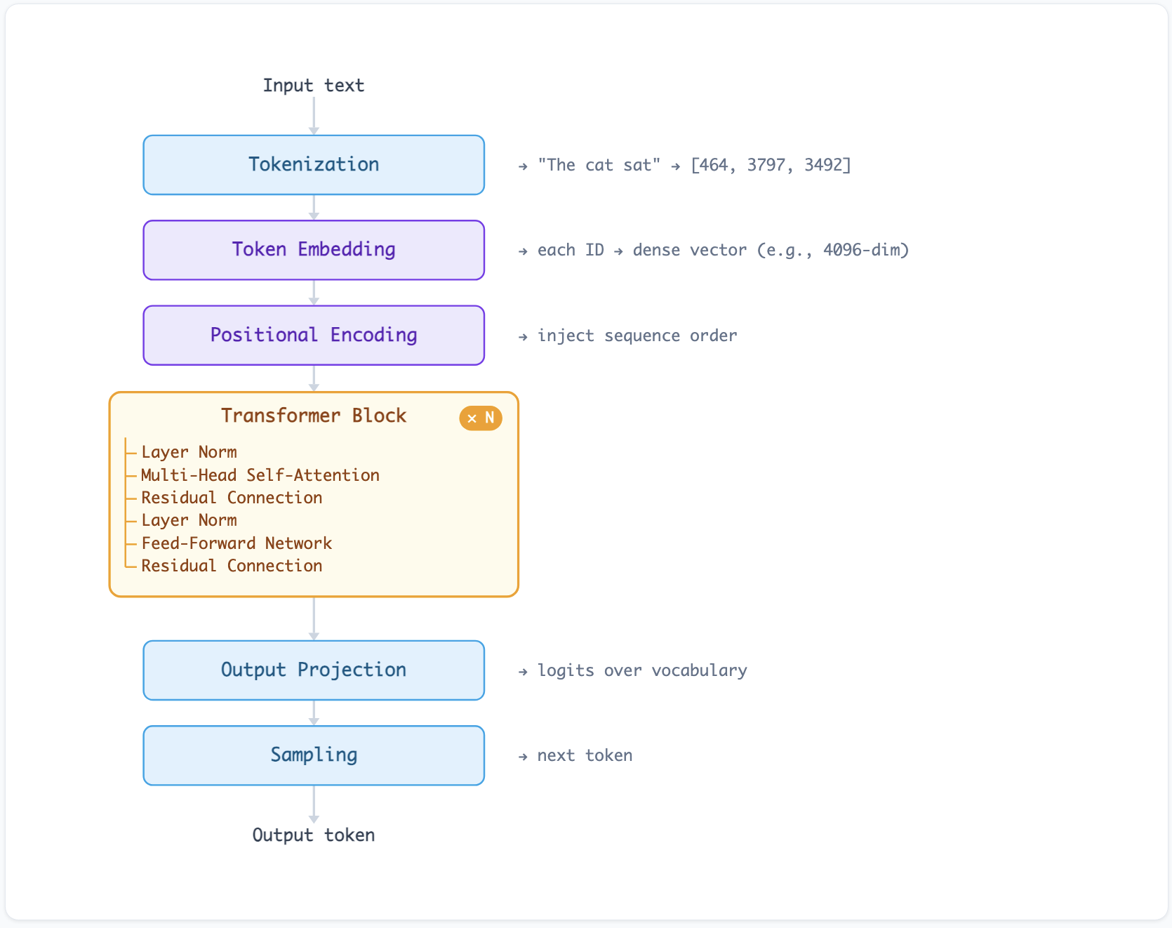
The rest of this article walks through each block.1
Tokenization: Text Becomes Numbers
Before the model sees anything, raw text is split into tokens, integer IDs drawn from a fixed vocabulary. This is not a neural operation. It is a deterministic preprocessing step.3
The key engineering fact: tokenization determines cost. Every token consumes compute through every layer of the model. A prompt that tokenizes into 500 tokens costs roughly twice what a 250-token prompt costs, both in latency and in API billing. The multilingual tax is real: the same semantic content in Tamil can cost 7x more tokens than in English.2
Token Embeddings: IDs Become Vectors
Each token ID indexes into a learned embedding matrix. For GPT-3, this matrix has shape [50257 × 12288], where 50,257 is the vocabulary size and 12,288 is the model dimension. The lookup is a single matrix row selection. No computation, just retrieval.4
The resulting vector is dense and continuous. Tokens with similar meanings end up with similar vectors, but at this stage the similarity is static. The word "bank" gets the same embedding whether it appears in "river bank" or "bank account."5
Positional Encoding: Order Matters
Unlike RNNs, which process tokens one at a time and inherit order from the sequence itself, Transformers see all tokens simultaneously. Without intervention, "the cat sat on the mat" and "mat the on sat cat the" would produce identical representations.
Positional encodings fix this. The original Transformer used sinusoidal functions, mapping each position to a unique pattern of sines and cosines across dimensions. Modern LLMs typically use Rotary Position Embeddings (RoPE), which encode relative position through rotation in the complex plane. RoPE has a useful property: it degrades gracefully beyond training length, which is why some models can extrapolate to longer contexts than they were trained on.67
Position 0: "The"  → embed("The")  + pos(0)
Position 1: "cat"  → embed("cat")  + pos(1)
Position 2: "sat"  → embed("sat")  + pos(2)
The result: each token's representation now encodes both what it is and where it is. This combined vector enters the first Transformer block.8
Self-Attention: Tokens Talk to Each Other
Self-attention is the operation that makes Transformers work. It allows every token to look at every other token in the sequence and decide which ones are relevant to its current meaning.910
Each token is projected through three learned weight matrices into three vectors:11
- Query (Q): "What information am I looking for?"
- Key (K): "What information do I contain?"
- Value (V): "What information will I contribute?"
The dot product between a token's query and every other token's key produces a relevance score. High scores mean "pay attention to this token." These scores are normalized through softmax into a probability distribution, then used to take a weighted sum of value vectors.
The √dk scaling factor prevents dot products from growing so large that softmax saturates into a near-one-hot distribution. Without it, attention becomes brittle, attending to a single token and ignoring everything else.1213
In decoder-only models (GPT, Claude, LLaMA), attention is causal: each token can only attend to tokens that came before it in the sequence. This is enforced by masking future positions with negative infinity before the softmax, ensuring they receive zero attention weight. The model generates text left-to-right precisely because it can only look left.
Multi-Head Attention: Parallel Conversations
A single attention head asks one question at a time. Multi-head attention runs several heads in parallel, each with its own Q, K, V projection matrices. GPT-3 uses 96 heads. Each head learns to attend to different types of relationships.14
Research on BERT (Clark et al., 2019) found that individual heads specialize. Some track syntactic dependencies (subject-verb agreement across intervening clauses). Others follow coreference chains (linking "she" back to "Dr. Torres"). Others capture positional patterns (attending to the previous or next token). The model doesn't plan these specializations. They emerge from training.15
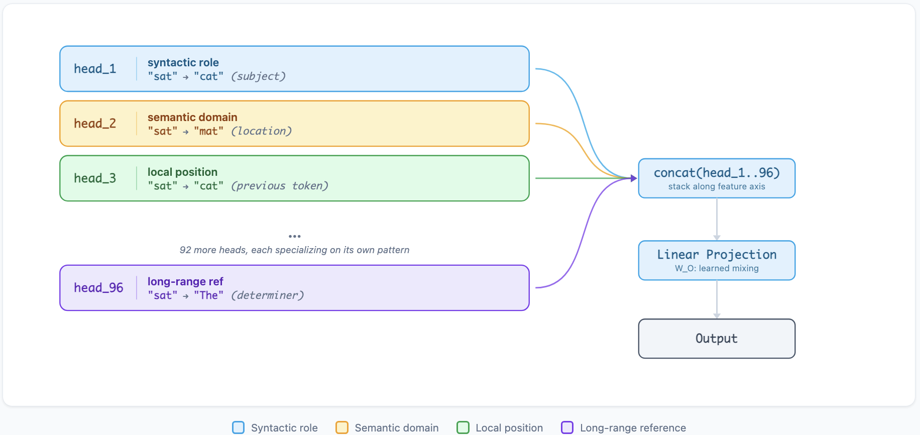
The outputs from all heads are concatenated and projected back to the model dimension. The result is a single vector per token that integrates information from 96 different "questions" about the sequence.
The Feed-Forward Network: Per-Token Processing
After attention, each token passes independently through a two-layer feed-forward network (FFN). This is the same network applied identically to every position:
The inner dimension is typically 4x the model dimension. For GPT-3, that's 12,288 in, 49,152 in the hidden layer, and 12,288 out. This expansion-compression pattern lets the network apply nonlinear transformations that attention alone cannot express.16
Recent interpretability work suggests the FFN layers function as key-value memories (Geva et al., 2021). The first matrix's rows act as keys matching input patterns; the second matrix's columns act as values that push the output toward particular next-token predictions. The FFN is where factual knowledge appears to be stored. When a model "knows" that Paris is the capital of France, that association likely lives in FFN weights, not in attention patterns.17
Residual Connections and Layer Normalization
Two mechanisms keep the signal stable across dozens of layers.
Residual connections add the input of each sub-layer back to its output: output = sublayer(x) + x. Without these skip connections, gradients vanish across 96 layers of computation. The residual stream gives gradients a direct path back to early layers during training, and gives the network a way to pass information through unchanged when a particular layer has nothing useful to add.
Layer normalization stabilizes activations by normalizing across the feature dimension. Most modern LLMs use Pre-Norm (RMSNorm before each sublayer) rather than Post-Norm (the original paper's approach), because it produces more stable training dynamics at scale.1819
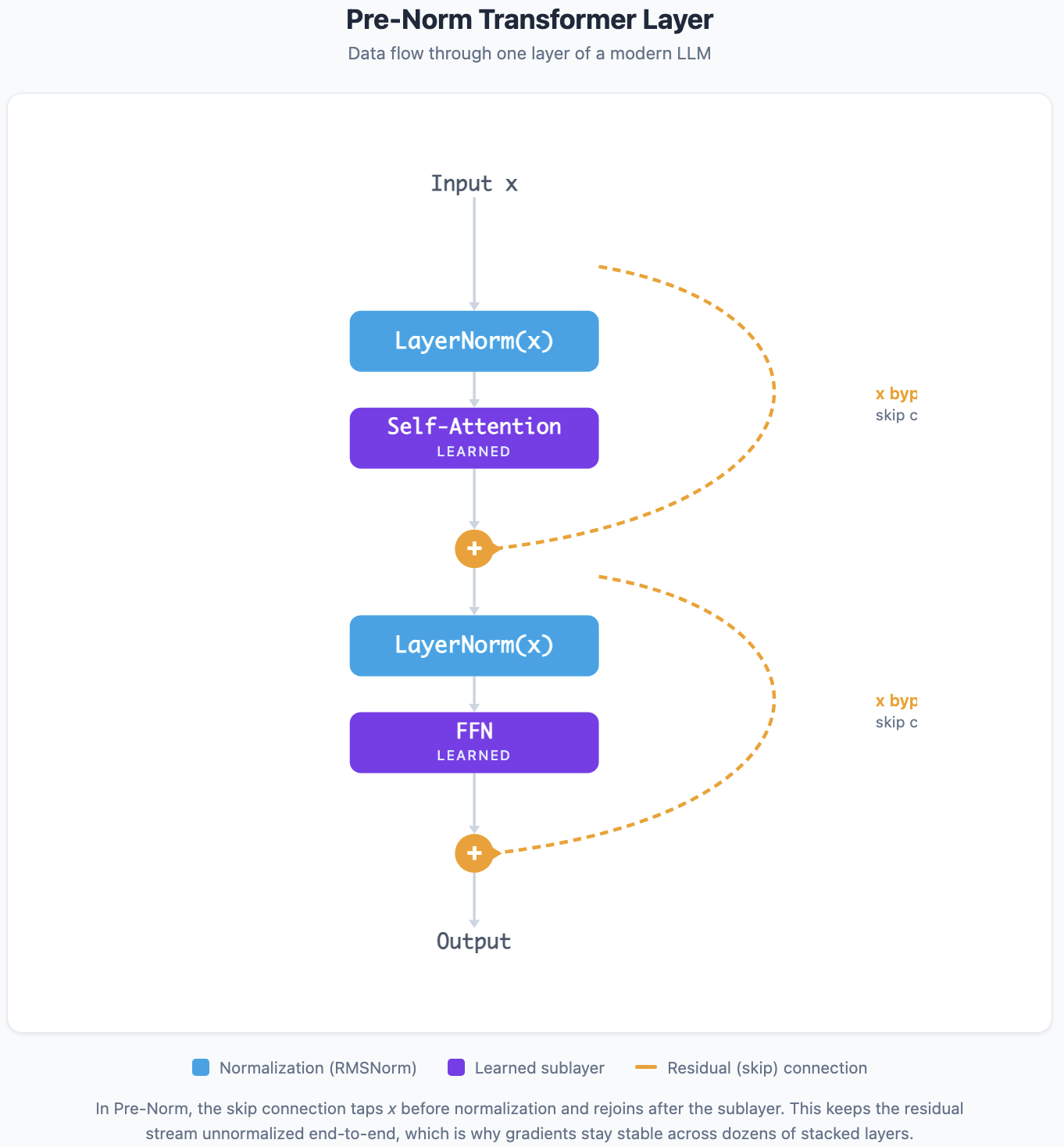
This pattern repeats for every layer. GPT-3 has 96 layers. LLaMA-70B has 80. Each layer's output feeds into the next, progressively refining the representation.
Output: From Vectors to Words
After the final layer, a linear projection maps each token's vector back to vocabulary size, producing logits, one score per possible next token. For GPT-3, this means a vector of 50,257 scores.
These logits are not probabilities. They become probabilities after softmax. But in practice, the sampling strategy you choose determines how those scores translate into text.20
Temperature divides the logits before softmax. Low temperature (0.1) sharpens the distribution toward the most likely token. High temperature (1.5) flattens it, giving unlikely tokens a better chance. At temperature 0, generation is deterministic.
Top-k keeps only the k highest-scoring tokens and redistributes probability among them. Top-k of 50 means the model chooses from its 50 best guesses.
Top-p (nucleus sampling) keeps the smallest set of tokens whose cumulative probability exceeds p. At top-p 0.9, the model dynamically adjusts how many tokens to consider. When one token dominates (95% probability), it selects from just a few. When the distribution is flat, it considers hundreds.2122
The selected token is appended to the sequence, and the entire process repeats. This is autoregressive generation: each token is conditioned on all previous tokens, one step at a time.
The KV Cache: Why Inference Costs Scale
Autoregressive generation creates an engineering problem. At each step, the model recomputes attention across the entire sequence. For a 1,000-token sequence, step 1,001 requires attending to all 1,000 prior tokens. Naively, this means recomputing Q, K, and V for every token at every step.
The KV cache eliminates redundant computation. Since previous tokens' keys and values don't change (the model only attends backwards), you compute K and V once per token and cache them. Each new step only computes Q for the new token, then attends to the cached K and V vectors.23
The tradeoff: memory. For GPT-3 with 96 layers and 96 heads, a 4,096-token sequence requires caching ~3 GB of KV pairs per request. This is why GPU memory, not compute, often limits how many concurrent requests a model can serve. It is also why longer context windows cost disproportionately more.24
Encoder-Decoder vs. Decoder-Only
The original Transformer had two halves: an encoder that reads the full input with bidirectional attention, and a decoder that generates output autoregressively with causal attention plus cross-attention to the encoder's output.
This architecture powers translation models (T5), summarization models (BART), and speech models (Whisper). You used both BART and T5 in DSCI-630 Week 1.
Modern LLMs chose a different path. GPT, Claude, LLaMA, and Gemini are decoder-only. They drop the encoder entirely and process everything, both input and output, as a single left-to-right sequence. Your prompt and the model's response are just one continuous sequence of tokens. The model doesn't distinguish "input" from "output" architecturally; the only difference is that prompt tokens are processed in parallel (prefill) while output tokens are generated one at a time (decode).
Why decoder-only? It simplifies scaling. One architecture, one training objective (next-token prediction), one set of weights. The encoder-decoder split makes sense when input and output have different structures (English to French). When the task is general text completion, the split adds complexity without clear benefit.2526
What This Means for LLM Engineering
Now that the machinery is visible, the six points from the opening are no longer claims but consequences. A concise recap, grounded in the components you just walked through:
Token count is compute cost
Every prompt token traverses every attention layer and every FFN. The cost is structural, not a pricing choice.
Context window is a hard boundary
Positional encoding and KV-cache capacity jointly define the maximum sequence length. Nothing attends past the edge.
Attention is global but weighted
Softmax concentrates probability on a handful of tokens. Middle-of-prompt context tends to lose weight against the head and tail.
Temperature is a softmax divisor
Low temperature sharpens the distribution; high temperature flattens it. The choice is precision versus variety, nothing more.
One token at a time
Each output token is a full forward pass over the cached KV context. Streaming is delivery order, not the model thinking aloud.
Behavior traces back to operations
Hallucinations, position bias, the drift near the context limit: every observed behavior maps to a specific operation in the stack.
The Transformer is a specific sequence of matrix multiplications, normalizations, and nonlinear activations, and every behavior you observe traces back to them.
References
Textbook grounding, chapter-level citations, and further reading for each numbered reference in this article live on the companion sources page.
- Vaswani, Ashish, et al. "Attention Is All You Need." Advances in Neural Information Processing Systems, vol. 30, 2017.
- Clark, Kevin, et al. "What Does BERT Look At? An Analysis of BERT's Attention." Proceedings of the 2019 ACL Workshop BlackboxNLP, 2019.
- Geva, Mor, et al. "Transformer Feed-Forward Layers Are Key-Value Memories." Proceedings of EMNLP, 2021.
- Su, Jianlin, et al. "RoFormer: Enhanced Transformer with Rotary Position Embedding." arXiv, 2021.
- Holtzman, Ari, et al. "The Curious Case of Neural Text Degeneration." ICLR, 2020.
Related Content
- The Elegant Hack Powering Modern AI (tokenization fundamentals)
- Breaking Text (BPE, WordPiece, SentencePiece, Unigram)
- The 30-Year Journey of BPE (algorithm history)
- Words Learning the Company They Keep (attention and disambiguation)
- The Hidden Geography of Language (embeddings)
- The Invisible Boundaries of AI Conversation (context windows)